Is Decoder Crowding Real, or Just Frequency in Disguise?

Steering a language model on a single sparse-autoencoder (SAE) feature is the clean version of interpretability's promise: find the "Golden Gate Bridge" direction, add it to the residual stream, and watch the model talk about bridges. The catch is collateral. Push on one feature and unrelated features light up too, and until you have run the model you do not know how much. A recent paper (Pre-Intervention Prediction of Sparse Autoencoder Steering Side Effects, Duan, arXiv:2606.08365) claims you can predict the mess in advance from geometry alone: a feature's decoder "crowding", how close its decoder direction sits to its neighbours, tracks the collateral damage better than the obvious baseline of how often the feature fires.

This is the second entry in a reproduce-then-probe series, and the probe here writes itself. Crowded features might simply be frequent features, so "crowding predicts collateral" could be "frequency predicts collateral" wearing a hat. The paper's headline does not run that control. So this notebook reproduces the result on GPT-2-small from scratch and then runs it.

What crowding is, and why it is cheap

Crowding is a pre-intervention quantity: it needs the SAE's decoder weights and nothing else, no forward pass. For each feature, take its decoder direction, measure the absolute cosine similarity to every other decoder direction, and average the top 20. A feature whose direction is nearly parallel to many neighbours is "crowded", and the intuition is that pushing along it inevitably drags those neighbours along.

Wn = torch.nn.functional.normalize(W_dec, dim=-1)          # unit decoder rows
sims = (Wn[chunk] @ Wn.T).abs()                            # cosines to all others
sims[torch.arange(len(chunk)), chunk] = 0.0               # exclude self
crowd = torch.topk(sims, 20, dim=-1).values.mean(-1)      # mean top-20 crowding

The whole appeal is that this costs a matrix multiply once, whereas measuring collateral for real means steering every feature and re-running the model.

Measuring the mess for real

To get ground truth, the notebook steers on GPT-2-small using Joseph Bloom's gpt2-small-res-jb SAEs, adding the feature's decoder direction at the final token of layer 8 and measuring what changes downstream at layer 10. Collateral is a count: over a 2,048-feature downstream panel, how many features shift by more than a threshold of 0.05, averaged over 48 contexts per feature. It samples 300 features (seed 0) from the non-degenerate firing band and correlates each cheap predictor against that measured collateral.

def steer(resid, hook):
    resid[:, -1, :] = resid[:, -1, :] + 1.0 * d_f          # push one decoder direction
    return resid
du   = (u_steer - u_clean)[:, panel].abs()
coll = (du > 0.05).float().sum(-1).mean().item()          # collateral spread

Crowding predicts, and the magnitude reproduces

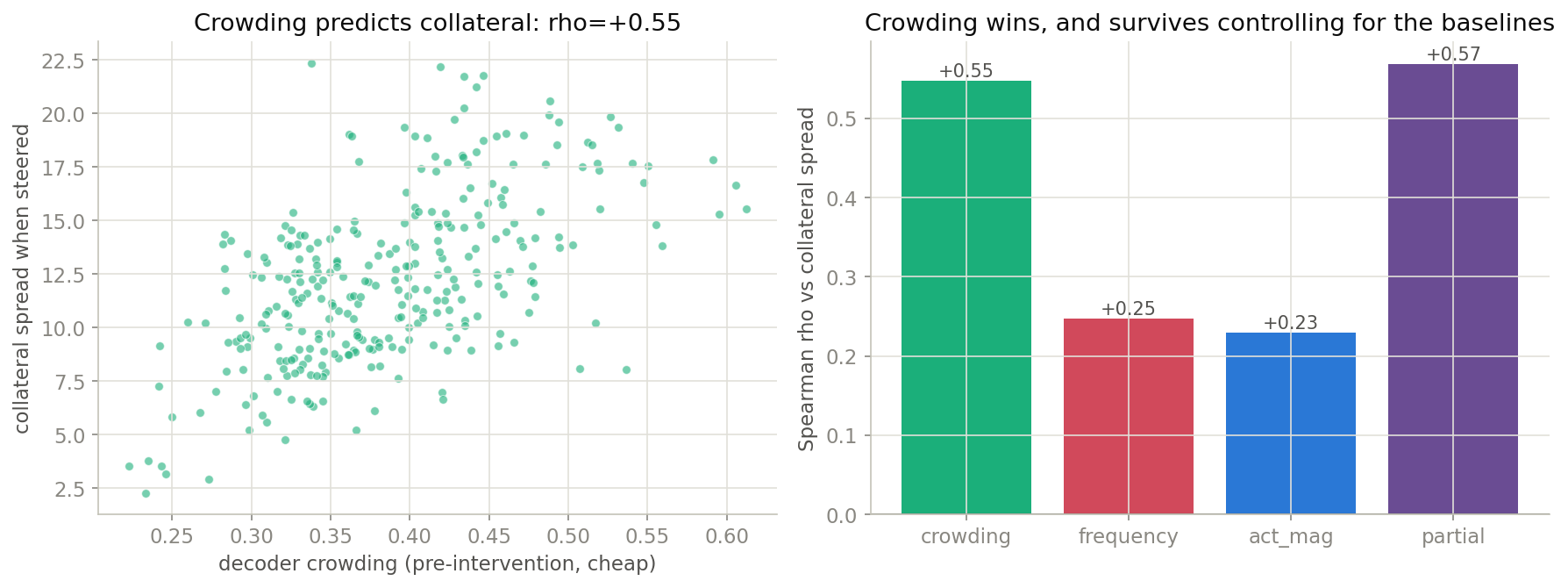
Across the 300 features, decoder crowding correlates with measured collateral at Spearman 0.55 (p = 6e-25), against the paper's reported ~0.47. Same sign, same order of magnitude, from an independent pipeline with its own steering and its own measurement. A property you can read off the decoder before touching the model tracks the damage steering actually causes.

The control the headline skipped

Now the probe. If crowding is just frequency in disguise, it should collapse once frequency is held fixed. It does not. Rank-transform crowding and collateral, regress out both firing frequency and mean activation magnitude, and correlate the residuals: the partial correlation is 0.57, if anything slightly higher than the raw 0.55. Crowding carries geometric signal that the firing-rate and magnitude baselines do not. It holds in both regimes too, 0.65 among rarely-firing features and 0.45 among often-firing ones, so this is not an artifact of one corner of the feature distribution.

Z = np.c_[rankdata(df["frequency"]), rankdata(df["act_mag"])]
partial_r, _ = pearsonr(_resid(rankdata(df["crowding"]), Z),
                        _resid(rankdata(df["collateral"]), Z))   # 0.57

predictor vs collateral spread      Spearman rho    paper
decoder crowding (raw)              0.55            ~0.47
firing frequency                    0.25            ~0
activation magnitude                0.23            -
crowding | frequency + magnitude    0.57            -
  low-firing half                   0.65            -
  high-firing half                  0.45            -

That the partial correlation matches the raw one is the result that convinces, more than the raw margin does. The skeptic's hypothesis is not weakened, it is rejected.

The honest divergence

The reproduction is directional, not bit-exact, and the gap is worth naming. The paper reports firing frequency as essentially useless, a correlation near ~0. Here frequency predicts collateral at 0.25, weak but clearly nonzero. So crowding's margin over the frequency baseline is +0.30 in this run, smaller than the paper's +0.43 to +0.47. The leading suspect is the steering coefficient: this notebook uses a fixed alpha of 1.0, while the released code uses a per-run global scalar tied to the activation distribution, which would change how hard each feature is pushed and therefore how much of the frequency signal leaks into collateral. The winner is the same in both; the size of its lead is setup-dependent, which is exactly why the control matters more than the margin.

Scope and limits

It reproduces the paper's central GPT-2-small mechanism from scratch, using its SAE and metric definitions cross-checked against the released code, and it stress-tests the mechanism with a partial correlation the headline did not foreground, which crowding passes. It does not match the paper's exact margin, does not test larger models or other SAE families, and does not establish why crowded directions bleed into their neighbours. The value is the control: a cheap, pre-intervention geometric property predicts steering collateral, and that predictive power is not a repackaging of how often the feature fires.

---

Runs end to end on a free Kaggle T4. Run it yourself: the notebook on Kaggle. Paper under test: Pre-Intervention Prediction of Sparse Autoencoder Steering Side Effects, Duan, arXiv:2606.08365. Model GPT-2-small with the gpt2-small-res-jb SAEs, steering at layer 8 and measuring at layer 10, 300 features sampled at seed 0.